Nearest neighbour spacing distribution in the GUE

This is an evaluated Mathematica notebook. Since the notebook is intended to be interactive, it may be helpful to also view the unevaluated version

Power series expansion of the d.e. about the origin

In[1]:= Out[1]=

     3       5        6          7          8                  2   9          10                2   11
   -s       s        s          s          s       (-350 + 3 Pi ) s      491 s        (1694 - Pi ) s
  ----- + ------ - ------- - -------- + -------- + ----------------- - ------------ + ----------------
  12 Pi   360 Pi         2   20160 Pi          2                3                 2                3
                   432 Pi               5400 Pi       5443200 Pi       63504000 Pi     239500800 Pi

Power series expansion of nn(s) about s=0

In[2]:= Out[2]=

      2  2       4  4       6  6        6  7         6              5       7               8  9
  2 Pi  s    4 Pi  s    2 Pi  s    32 Pi  s     -8 Pi          -4 Pi    2 Pi     8   2144 Pi  s
  -------- - -------- + -------- - --------- + (------ - 2 Pi (------ + -----)) s  + -----------
     3          45        315        2025        243            243     14175          496125

Numerical solution of the d.e., calculation
of the mean and comparison with power series
expansion

Here the power series solution at s=1.1 is used as the
initial condition

In[3]:=

Out[3]=

  {{y -> InterpolatingFunction[{1.1, 16.}, <>]}}

In[4]:=

Here the numerical solution is integrated to
determine the mean of the distrubution

In[5]:=

Out[5]=

  0.725227

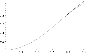
Next the numerical solution is compared to the power series solution

In[6]:=

Out[7]=

  -Graphics-

The function nn(s) can be tabulated

In[8]:=

In[9]:= In[10]:=

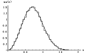
Comparison with data from the GUE

Code to generate GUE matrices and plot empirical value of nn(s) (output suppressed)

In[11]:=

In[12]:=

If your output will be a sequence of graphs, select a display option.
Display as:

In[13]:= In[14]:= Calculation of theoretical curve for nn(s) and comparison with numerical data

In[15]:=

In[16]:= In[17]:=

Out[18]=

  -Graphics-

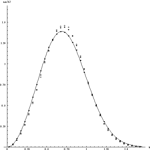
Comparison with data from zeros of Riemann
zeta function for 10^6 zeros about the 10^20
zero, 10^6 zero and first zero

Here we read in the data as a list. The data gives the number
of zeros in the intervals [j*.05, (j+1)*.05) (j=0,...40). The third,
fourth and fifth columns contain the data for zeros about
zero 1, zero 10^6 and zero 10^20 respectively. The theoretical
value of nn(s) is plotted from the Table t.

In[19]:=

In[20]:=

Out[21]=

  -Graphics-