4. Shaded Nullclines and Single ODEs

Finally, I would like to show how the shaded region idea can be profitably used for single ODEs. In such a case one might shade the background according to the slope of the underlying slope field, perhaps with a superimposed thicker curve on the 0-isocline, which separates the regions of positive and negative slope. This sort of shading is discussed by Hubbard and West [HW, p. 16], who say that such a "color-coding method takes a little getting used to." I think that the addition of a thick curve for the 0-isocline makes this type of image somewhat clearer.

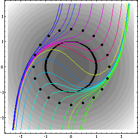
While such isocline shading is certainly easier to accomplish with the VisualDSolve package, it can be done from scratch using Mathematica's contour plotting and DE-solving tools, and we now show how. But first take a look at the stunning image that results. The thick black line separates the regions of positive and negative slope; the dots are the initial values.

To get the image, we first define the equation. But we introduce an If statement so that it returns a number only if x is between -2.5 and 2.5; this forces the numerical DE solver to shut off outside the viewing window. It will generate some warning messages when this happens, which we suppress with Off; this technique increases efficiency by avoiding computations ourside the viewing window.

In[27]:=

Next we create the shaded background by making a contour plot of the right-hand side of the equation. To get inside the If, we use equation[[2, 2]], and we replace x[t] by x to get an expression in x and t to send to ContourPlot. The ColorFunction will get normalized arguments between 0 and 1, and so the pure function "# 0.6 + 0.4" will take on values between 0.4 and 1, giving us nice soft shades of gray. The Identity setting suppresses the display.

In[28]:=

Now the single thick nullcline is generated in much the same way, with ContourShading turned off and with Contours set to the single value 0.

In[29]:=

Next we set up some initial values in the shape of a circle and feed them to NDSolve. Thus solutions as defined below will be a list of 21 interpolating functions.

In[30]:=

We now generate plots of these solutions, using a Hue setting that varies with the solution.

In[31]:=

Finally, we show the whole business in the right order, together with some points at the initial values. Of course, we must set the DisplayFunction to override all the suppressions of the preceding graphics work.

In[32]:=

equation = x'[t] == If[Abs[x[t]] <= 2.5, x[t]^2 + t^2 - 1];
  Off[NDSolve::ndnum];
  
  shadedBackground = ContourPlot[
    equation[[2, 2]] /. x[t] -> x, {t, -2.5, 2.5}, {x, -2.5, 2.5},
      Contours -> 15, ContourLines -> False, PlotPoints -> 40,
      ColorFunction -> (GrayLevel[# 0.6 + 0.4]&),
      DisplayFunction -> Identity];
  
  thickNullcline = ContourPlot[
    equation[[2, 2]] /. x[t] -> x, {t, -2.5, 2.5}, {x, -2.5, 2.5},
      Contours -> {0}, ContourShading -> False, PlotPoints -> 40,
      ContourStyle -> {Thickness[0.015]},
      DisplayFunction -> Identity];
  
  initialVals = Table[1.5 {Cos[t], Sin[t]}, {t, 0, 2 Pi, N[Pi]/10}];
  
  solutions = x[t] /. Map[First[
    NDSolve[{equation, x[#[[1]]] == #[[2]]}, x[t], {t, -2.5, 2.5}]]&,
    initialVals];
  
  solutionImages = Table[
    Plot[Evaluate[solutions[[i]]], 
      {t, solutions[[i, 0, 1, 1]], solutions[[i, 0, 1, 2]]},
      PlotStyle -> {{AbsoluteThickness[2], Hue[1 - 0.8 i/21]}},
      DisplayFunction -> Identity],  {i, 21}];
  
  Show[{shadedBackground, thickNullcline, solutionImages}, 
  Graphics[{PointSize[0.02], Map[Point, initialVals]}],
  DisplayFunction -> $DisplayFunction, AspectRatio -> Automatic];

If your output will be a sequence of graphs, select a display option.
Display as:

Bug fix

The above is a little involved. Here is how our package, VisualDSolve, can be used to generate the same image with one call to VisualDSolve.

In[34]:=

Up to New Visualization Ideas for Differential Equations