In[8]:=
Out[8]The root is returned in the form of a substitution rule. We can define rx and ry to be the x and y coordinates of the root, and then we plug into the given functions as a check (% refers to the preceding output).
In[9]:=
Out[9]
So far, so good. But our problem here is a little different in that we want to
know all the equilibrium points in a given rectangle. Here is where the power of
Mathematica, and its openness in allowing us access to the data in a
contour plot comes into play. Consider the following algorithm:
1. Generate the curve(s) representing f = 0 by using a contour plot for the 0
contour.
2. Evaluate g along the curves, and check for sign changes of g.
3. Since a sign change of g along f = 0 means that we are quite close to a
root,
we can use the gathered values as seeds to FindRoot.
In fact, this procedure works very well and is not too difficult to program.
The function Equilibria which accompanies this article implements it in detail.
Since the main outline is so simple, we illustrate the programming methodology
by following through an example. Graphics[ContourPlot[***]] returns a
complicated graphics object that has imbedded in it the several Line objects
making up the contours. Cases[***, _Line, Infinity] picks them out no matter
where they are. First then strips off the Line header because we are really
interested in these objects as lists. We reintroudce the Line headers in order
to confirm visually that this scheme has worked.
In[12]:=
Out[12]Good. We now have the five curves as lists in contourData. Let us now focus on the central curve, given by contourData[[5]]. We apply g and look at the signs of the result.
In[13]:=
Out[13]Multiplying this vector by a shift of it causes the sign-changes to show up as -1s. There are six of them.
In[14]:=
Out[14]We now find the places in the plane where these sign-changes occurred.
In[16]:=
Out[16]This gives us six approximations. We define a function, root, that feeds a single seed to the rootfinder; mapping this function to the set of seeds produces six fairly exact roots.
In[17]:=
Out[17]=
  {{x -> -9.0854, y -> 3.02456},

    {x -> -6.70018, y -> 2.71369},

                     -23
    {x -> -6.36474 10   , y -> 0.},

    {x -> -3.80395, y -> -2.33935},

    {x -> -5.81937, y -> -2.60337},

    {x -> -9.75079, y -> -3.1229}}
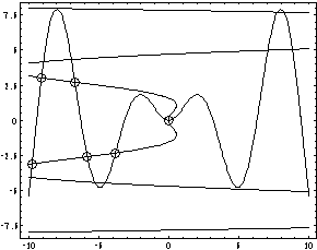
The following figure, which shows the contours together with circles around the data we just found, shows that the approach has worked beautifully and we have found all six solutions on the central contour.
In[18]:=
As mentioned, Equilibria implements this in general. It finds all 16 equilibria points for our example in short order.
In[19]:=
Out[19]
There are some options to Equilibria. Setting SeedsOnly to True causes just the
seeds to be returned. The EquilibriaPlotPoints option controls the number of
plot points in the contour plots that get the algorithm started; for difficult
examples this might have to be increased from the default of 49. And there is a
ShowEigenvalues option that produces a table of the equilibrium points together
with the eigenvalues of the Jacobian at the points.
EXERCISE. Modify these ideas to get a routine that finds all complex roots of a
complex function f(z) in a given rectangle. Just apply the same method, looking
at f's imaginary part along a contour plot of the real part. FindRoot, does in
fact work on complex functions, provided I appears in either the function or the
initial value.