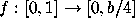
 is defined by
 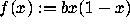 , where
  .
The points x=0 and
.
The points x=0 and  are both fixed points
of the map. Unlike the linear map,
calculating the Lyapunov exponent is not trivial
since the derivative
are both fixed points
of the map. Unlike the linear map,
calculating the Lyapunov exponent is not trivial
since the derivative 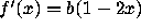 is not constant for the map. We can, however, do a few
computational experiments to better understand this map.
is not constant for the map. We can, however, do a few
computational experiments to better understand this map.
The following links call up the Maple Form Interface. All
the examples considered involve the case b=4, so
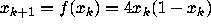 . Please read the
explanations in this document before calling up
the Maple Form Interface so that you can be clear
on what each section of code is actually doing.
(Of course, if you are familiar with Maple,
you can decipher the code easily.)
. Please read the
explanations in this document before calling up
the Maple Form Interface so that you can be clear
on what each section of code is actually doing.
(Of course, if you are familiar with Maple,
you can decipher the code easily.)
 which
is a fixed point of this map. What happens to the
orbit of y0 when y0 is close to
which
is a fixed point of this map. What happens to the
orbit of y0 when y0 is close to  ?
Try changing x0 and y0 to see how orbits of
other neighbouring points behave. (If you increase N,
bear in mind that the output may not be easy to read.)
?
Try changing x0 and y0 to see how orbits of
other neighbouring points behave. (If you increase N,
bear in mind that the output may not be easy to read.)
 and
N=50. Increase N to make a reasonable guess
as to what the Lyapunov exponent
and
N=50. Increase N to make a reasonable guess
as to what the Lyapunov exponent  is.
Change x0 to 0, 0.75 and other values in [0,1]
to see how the approximation
is.
Change x0 to 0, 0.75 and other values in [0,1]
to see how the approximation
 varies.
 , Maple returns the number
of iterations required for the separation between
orb(x0) and orb(
, Maple returns the number
of iterations required for the separation between
orb(x0) and orb( ) to be multiplied
by 10. Initially, the values
) to be multiplied
by 10. Initially, the values  and
and
 are used; try changing them. Is
there any pattern emerging?
are used; try changing them. Is
there any pattern emerging?
![[Shownotes]](../gif/annotate/shide-31.gif)