
 Comparison with the analogous expansion of (1.3a) (see e.g. [2]) shows that
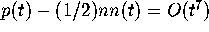 , which in qualitative terms says that
very small spacings between consecutive eigenvalues will most likely be
nearest neighbour spacings (the factor of 1/2 accounts for the fact that the
nearest neighbour occurs with equal probability to the left or the right).
, which in qualitative terms says that
very small spacings between consecutive eigenvalues will most likely be
nearest neighbour spacings (the factor of 1/2 accounts for the fact that the
nearest neighbour occurs with equal probability to the left or the right).
 (see e.g. [7]) and seek a solution of the form
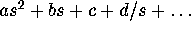 . Indeed (2.7) has a unique solution of this
form, which when integrated according to (2.6) implies
. Indeed (2.7) has a unique solution of this
form, which when integrated according to (2.6) implies

 As is well known (see e.g. [7]) this leaves the overall multiplicative constant
A unspecified. The large-t expansion of
As is well known (see e.g. [7]) this leaves the overall multiplicative constant
A unspecified. The large-t expansion of  is obtained by substituting
(3.2) in (2.4).
The solution of (2.7) with b=1 was computed numerically by first calculating
the power series expansion of
is obtained by substituting
(3.2) in (2.4).
The solution of (2.7) with b=1 was computed numerically by first calculating
the power series expansion of  up to
up to  and using the
corresponding values of
and using the
corresponding values of  and
and  as initial data in
the
Mathematica routine NDSolve.
The d.e. (2.7) was rewritten so that
as initial data in
the
Mathematica routine NDSolve.
The d.e. (2.7) was rewritten so that  occured to
the first power (the negative square root is to be taken) and it was found
necessary to use a high precision setting (AccuracyGoal and PrecisionGoal = 20) to
get a stable solution in the interval of interest (s < 13).
occured to
the first power (the negative square root is to be taken) and it was found
necessary to use a high precision setting (AccuracyGoal and PrecisionGoal = 20) to
get a stable solution in the interval of interest (s < 13).
Although the results of Section 2 are only exact in the limit  , it is well known that
  can be accurately approximated by
considering
can be accurately approximated by
considering  matrices which give the so called Wigner surmise
(see e.g. [2]). This suggests that
matrices which give the so called Wigner surmise
(see e.g. [2]). This suggests that  may also be insensitive to the
precise dimension of the GUE matrices. Assuming this, to test our exact
expression we have compared
may also be insensitive to the
precise dimension of the GUE matrices. Assuming this, to test our exact
expression we have compared  as calculated from (2.6) with
 as determined empirically from 10,000 numerically generalted
 matrices from the GUE (see
Figure 1
). The latter calculation was done using
Mathematica. For each matrix the eigenvalues were calculated
and the nearest neighbour spacing of the middle (8th) eigenvalue was
calculated. After scaling the spacings were tested to count how many fell
into the intervals
matrices from the GUE (see
Figure 1
). The latter calculation was done using
Mathematica. For each matrix the eigenvalues were calculated
and the nearest neighbour spacing of the middle (8th) eigenvalue was
calculated. After scaling the spacings were tested to count how many fell
into the intervals 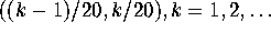 , and the corresponding
empirical value of
, and the corresponding
empirical value of  plotted at the points
 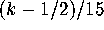 .
.
![[Shownotes]](../gif/annotate/sshow-71.gif)
![[Shownotes]](../gif/annotate/sshow-72.gif)