
Contents
Next: The balancing transformation.
Up: The Prüfer Transformation
Previous: The Prüfer Transformation
Analyzing  for the Airy equation.
![[Annotate]](/organics/icons/sannotate.gif)
![[Shownotes]](../gif/annotate/sshow-31.gif)
If the Airy equation  is transformed into a
system of the form (2) in the standard way, setting
  , we obtain
the linear time-dependent system


The Prüfer transformations are then applied to the Airy equation, as
represented by system (8), equation (6) becomes


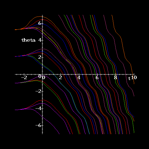
Trajectories of this equation are shown in Figure 2. In the left
half-plane, various funnels and antifunnels are visible, but they do not
give any better information than the Ricccati equation (16).
The solutions on the right of Figure 2 seem to be merging
(far offscreen) as  ,
but they are too wiggly for us to be able to find good fences
for a funnel or antifunnel argument.


Figure 2: Trajectories for equation for  , before balancing.


Contents
Next: The balancing transformation.
Up: The Prüfer Transformation
Previous: The Prüfer Transformation
 for the Airy equation.
 for the Airy equation.
 is transformed into a
system of the form (2) in the standard way, setting
  , we obtain
the linear time-dependent system


 ,
but they are too wiggly for us to be able to find good fences
for a funnel or antifunnel argument.


 , before balancing.