 after balancing.
 after balancing.
 ,
and they are ``straight'' enough to try using the
theory of fences and funnels.
In fact, as a result of Condition II, we see from equation (12) that as
 , solutions are going to behave very much like solutions to
the equation
  . To be precise, from (12) we get

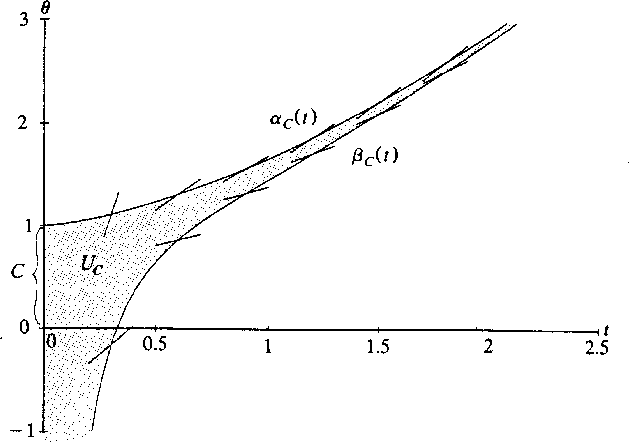
 for all t > 0. Therefore, for any C, the curves

 are respectively a lower fence and an upper fence for the differential
equation (12). That is, for every t>0 the slope
  the slope of the direction field for
  at that point, and
 the slope of the direction field. Together these fences
define an antifunnel
 , which is narrowing as
  ; see Figure 5.
We will show in Appendix C that there is exactly one solution
 which is trapped in the narrowing antifunnel
  for all
t>0, and that every solution of (12) for t > 0 is of this form for
some C.


 and
and  forming the antifunnel
  for equation
 .
.

These facts allow us to determine the spacing of the zeroes of  .
Recall that
  ,
so
,
so  if and only if
  is an odd multiple of
  .
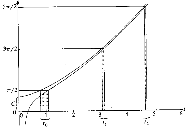
Figure 6 shows the
t-intervals in which the zeros of
  must lie;
that is, the intervals between the curves
  and
and  corresponding to equally spaced values of
  .
.


Figure 6: The t-intervals trapping the zeroes of  ; here
 .
.

Let  denote the zero of
  correponding to
  . Since the solution
  stays inside the
antifunnel
  , it is clear that the interval defining
  shrinks
as
  ; in fact, for large n we have

 Hence (l'Hôpital) the distance
  between successive zeros
approaches
0 as
  . So our intuition that the oscillations are more and
more compressed, and that the distance between successive zeros goes to
zero as
  , was correct!