Contents Next: A backwards antifunnel. Up:A New Look at Previous: What Happens for

The Riccati Transformation

The Riccati substitution

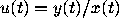
transforms the linear time-dependent system (2) into a first-order nonlinear ordinary differential equation in the single variable u:

Equation (15) is known as the Riccati equation associated with the system (2).

The Riccati equation associated with the system (8) associated with the Airy equation is

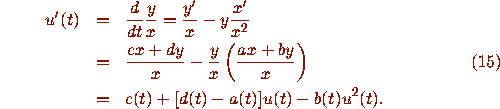
A picture representing the slope field, and several trajectories, of equation (16) is shown in Figure

Figure 8: Trajectories for the Riccati equation associated with the Airy equation.

It is clear from Figure that the left half-plane t < 0, corresponding to the region of the xt-plane in Figure where trajectories seem to be non-oscillatory, is more amenable to analysis, because solutions appear to funnel together or spray apart. In fact, this is a mirror image (about the u-axis) of the phase plane analyzed by John Hubbard in [3]. Since all of this deals with question 2, we shall defer further discussion until we have dealt with question 1: the behavior of the solutions for t > 0. The oscillatory solution for t>0 shown in Figure suggests that we try the Prüfer transformation.

We redraw Figure as Figure , adding isoclines of slopes -1, 0, +1. Portions of these three isoclines act as fences to form funnels and antifunnels.

Figure 9: Trajectories for the Riccati equation , with isoclines of slopes -1, 0, +1.

Contents Next: A backwards antifunnel. Up:A New Look at Previous: What Happens for